
A crash course into digital audio representation
So how does sound work?
Sound—as we all know—is a longitudinal (or compression) wave through some medium; generally air. These pressure waves are created when an object vibrates, which creates an alternating low and high pressure near the vibration. As these pressure differences occur, they pull and push the particles near them, causing a ripple effect of air pressure changes. This compression wave travels longitudinally; that is, no single particle travels with the wave, but rather, the particle bumps into another particle that’s a bit further along on the wave and transfers the energy onto this next one, which then bumps towards another particle a bit more further, eventually propagating most of this energy along in the direction of the wave.
Once this pressure wave reaches our ears, the changes in air pressure equally cause the eardrum to vibrate, which is then converted by a very intricate process into signals that eventually make it into our temporal lobe where we recognise those sounds. Humans generally perceive sounds between 20 Hz and 20 kHz. Hertz (Hz) is the unit generally used for frequency; it is the number of “full waves” per second. The amplitude of a wave is the “size” of the wave, in this case, it’ll be half the difference between the maximum pressure and minimum pressure sections of the wave. Sound through air travels roughly at a constant speed of \(343\ \text{m}/\text{s}\), so knowing the frequency dictates the wavelength.
Sound is therefore characterised by two important factors: the frequency of the wave, and the amplitude of the wave. In practice, however, sound doesn’t come in a single-frequency, pure wave; but is rather a combination of several waves of slightly different frequencies, due to several other non-fundamental normal modes discussed in the next section. Furthermore, because of several factors—such as the medium dispersing and distorting the wave—the pressure wave isn’t always a perfect sine wave, and so it’s often not enough to simply measure the frequency and amplitude.
Fundamental frequencies and harmonics

Imagine for a moment plucking a guitar string so that it starts vibrating. How exactly does it vibrate? One can clearly see that the string is vibrating back and forth, with the middle parts of the string moving further away from their “resting” position than the ends which are rather fixed. Comparing to the image above, what we see is probably along the lines of the first wave. This wave is called the first normal mode of the string; and the frequency at which the string vibrates depends on the tension, mass, and length of the string. This is the most natural vibrating motion for the string, and gives rise to the lowest frequency observed, called the fundamental frequency.
However, often the string will also vibrate at other frequencies. Looking again at the illustration, there are several standing waves that can form for the same length of string. These standing waves make up the different normal modes of the string. A drum on the other hand, won’t vibrate like a string, but has a much more complex set of normal modes; of which some can be solved for by the Bessel function. The normal mode with lowest frequency is the fundamental frequency and the other normal modes give to what are known as harmonics, or overtones.
Every instrument has a slightly differing profile of frequencies that they produce for a given note—even when that note has the same pitch—and these are a large part of what give instruments their unique sound: their timbre, or tone colour (the other half is the envelope of the sound, which describes roughly variations in the long-timeframe amplitudes of the sound). The normal modes of an oscillator depend on the shape and other properties of it, for instance, woodwind instruments have one unconstrained end at the end of the column, so their normal modes will differ from those of string instruments whose both ends are fixed.
Measuring sound
Now that we’ve had a quick reminder to how sound works, the next question follows: how do we represent this sound digitally? We must obviously measure the air pressure (or rather, the difference between the air pressure and the ambient air pressure), and then store these pressure readings. This leads naturally to a few central questions: how often do we have to measure the air pressure, and how well do we have to measure it?
The Nyquist-Shannon sampling theorem
The answer to the former has a particularly satisfying answer through a much celebrated result in mathematics; the Nyquist-Shannon sampling theorem. Assume now for a moment that the pressure wave were indeed a perfect sine wave. It’s possible to mathematically prove that to perfectly capture any sine wave of frequency \(f\) Hz, it suffices to sample every \(1/(2f)\) time units, that is, the sampling frequency needs to be \(2f\) Hz. Thus, if one has sound whose every frequency lies below \(f\) Hz, then it suffices to sample at a rate of \(2f\) Hz.
In particular, the fundamental frequency of a human is normally within the range of 85 Hz to 255 Hz. However, it turns out that due to overtones, it is easy to make out what they are saying even if these frequencies aren’t perfectly reproduced. Furthermore, normal human speech rarely reaches a few thousand hertz. This gives rise to the voice frequency band (VF), which is approximately between 300 Hz and 3400 Hz. Furthemore, the Nyquist-Shannon sampling theorem tells us that to then reproduce this sound, we need to only sample at a rate of 8 kHz. So mobile phones, landlines, and most rudimentary devices that deal with exclusively human voices mostly care about reproducing this band of sound most faithfully while possibly sacrificing other frequency bands, and in situations with limited resources, one often finds simple encodings with a sampling rate of 8 kHz.
This is exactly the reason why classical music sounds absolutely abysmal as hold music! The technology was never aimed at faithfully reproducing the high frequencies of violins and other orchestral instruments. Even if they were able to fully capture the fundamental tone, they’ll completely fail at reproducing the overtones, which are vital for hearing the complex sounds of these instruments.
So just to recap: if we sample at a rate of \(2f\) Hz, then we will be able to reproduce every perfect sine wave with frequency less than or equal to \(f\) Hz—this is called the Nyquist rate of the frequency.
Sampling resolution, or bit depth
The other important part of converting an audio signal into digital form is the bit depth of each sample. This measure refers to the number of bits used to store each sample. Clearly then a larger number of bits allows a more faithful reproduction of the exact amplitude of the sound wave at each sampling epoch.
Commonly audio is stored at a bit depth of 16, 20, or 24 bits, and occasionally 32 bits for professional audio or during editing—the additional bit depth helps mitigate issues with rounding and errors with the smaller bit depth, even if the audio is in the end reduced to 16 bits per sample. In particular, audio on CDs for instance is stored at 16 bits per sample.
Recall that one can store at most 256 different values in 8 bits of memory. This gives rise to the familiar tone of the 8 bit music you might remember from some old video games. 16 bits of memory can store at most 65536 different values, and so forth such that \(n\) bits of memory can store at most \(2^n\) distinct values.
Linear Pulse Code Modulation
Naturally, the next question is then; what should we store in those precious \(2^n\) values?
Maybe the most obvious idea is this: call the value of the highest magnitude of your signal \(A\), and divide the range from \(-A\) and \(A\) evenly into \(2^n\) quantisation steps. Now take your recording, and for every sample approximate it with the closest quantisation level. This is called Linear Pulse Code Modulation, or LPCM for short. Linear means that every step is an even distance away, and Pulse Code Modulation is the process of approximating the magnitude of the signal with one of the predetermined quantisation steps. The first obvious drawback of this method, however, is that we won’t always know the largest amplitude of the signal as we start recording. It turns out that this is relatively easily fixed by just choosing the right gain level, or using an Automatic Gain Control mechanism.
Maybe the most common audio representation is 16-bit PCM, which is just using 16-bit signed integers with LPCM to represent samples.
Another more nuanced drawback of this method is that this way of assigning the discretisation steps of the signal is probably not the best one. If most of the time the amplitude of the signal is close to zero, then it’d make sense to have a more accurate representation of amplitudes near zero by assigning some precious discretisation points there, rather than evenly spreading them out everywhere.
If you’re from a software engineering background, the first idea you’d probably come up with would be to use floating point number to represent your signal. Floating point number approximate values near zero very closesly, and as one moves further away from zero, the quantisation error increases. This gives—in the context of audio—more than enough range to represent samples in. This is indeed something used in some circles of professional audio, where being a little wasteful with the bit depth is not so important.
However, there’s—debatably—an even better way of discretising the amplitude levels. The idea here is to look at the distribution of samples, and compute the optimal discretisation points. This is exactly the idea behind the A-law and the µ-law companding algorithms.
Companding: the A-law and the µ-law
Companding is just a funny way of joining “compressing” and “expanding”, and is exactly that: it’s when you compress your signal at the transmitting end, and expand it at the receiving end.
The A-law and the µ-law are two very common ways of doing this; in particular in the domain of public switched telephone networks. The basic idea is this: human perception of sound is logarithmic, in the sense that we have a very hard time sensing a unit increase in amplitude, but rather sense in orders of magnitude. Furthermore, one can motivate these ideas by looking at the distribution of amplitudes in a normal recording of speech. It turns out that this distribution falls off almost logarithmically too, so it matches the idea of encoding common amplitudes more accurately than uncommon ones.
The compression function underlying the A-law for a given compression parameter \(A\) and a reading \(x\) with \(|x|<\frac{1}{A}\) is given by:
\[F(x)=\text{sgn}(x)\frac{A|x|}{1+\log(A)},\]
and for \(\frac{1}{A}\leq|x|\leq1\), it is given by:
\[F(x)=\text{sgn}(x)\frac{1+\log(A|x|)}{1+\log(A)}.\]
Here’s a plot of this function:
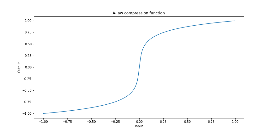
Note that the \(\log\) symbols here refer of course to the natural logarithm with base \(e\), and \(\text{sgn}\) is the sign function.
The µ-law compression function for a given \(\mu\) is similarly given for a reading \(-1\leq x\leq1\) by:
\[F(x)=\text{sgn}(x)\frac{\log(1+\mu|x|)}{\log(1+\mu)}s.\]
Here’s this function plotted as well:
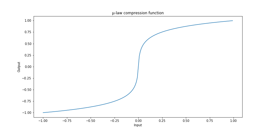
The basic idea of compression is then that we simply record our sample, pass it through this compression function, and store the closest linearly spaced value corresponding to that output.
The functions look very similar, but when we plot them near zero, we can see a small difference:
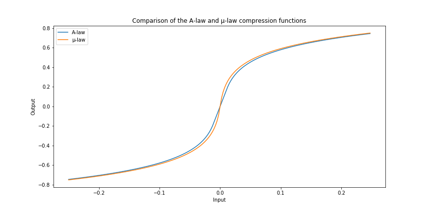
This small kink means that the µ-law method is ever so much accurate at representing the audio signal when it is quiet than the A-law algorithm.
In reality these two schemes are simplified even more: the compression functions are broken into a few piecewise-linear sections, further simplifying the compression and expansion algorithms; which may be crucial for performance on small embedded devices, a common use case.
Further concepts: audio compression and audio codecs
Of course, audio representation doesn’t end at simply picking a sampling rate, a bit depth, and doing the right companding. Often one wants to further compress the audio samples, and for this there are a plethora of different techniques. Most of these rely on the idea of trying to predict the next sample based on the past few samples, and only make slight corrections occasionally.
Audio compression algorithms are divided into two camps: lossy and lossless. Lossless obviously means that no information is lost when the audio is compressed: the bytes fed into the algorithm are precisely the same as those run through a roudn of compression and subsequent decompression. Lossy compression on the other hand allows some data loss; but this is generally managed by precise measurements and double-blind experiments on what kind of loss is acceptable and won’t produce notable differences in the perceived audio quality. MP3 for instance is based on the observation that upon encountering a certain mix of frequencies, the human ear only percieves a certain subset of those.