
Modeling NYC Taxi Profitability using a Leontief-style Model
This blog post is joint work with Alex Huang.
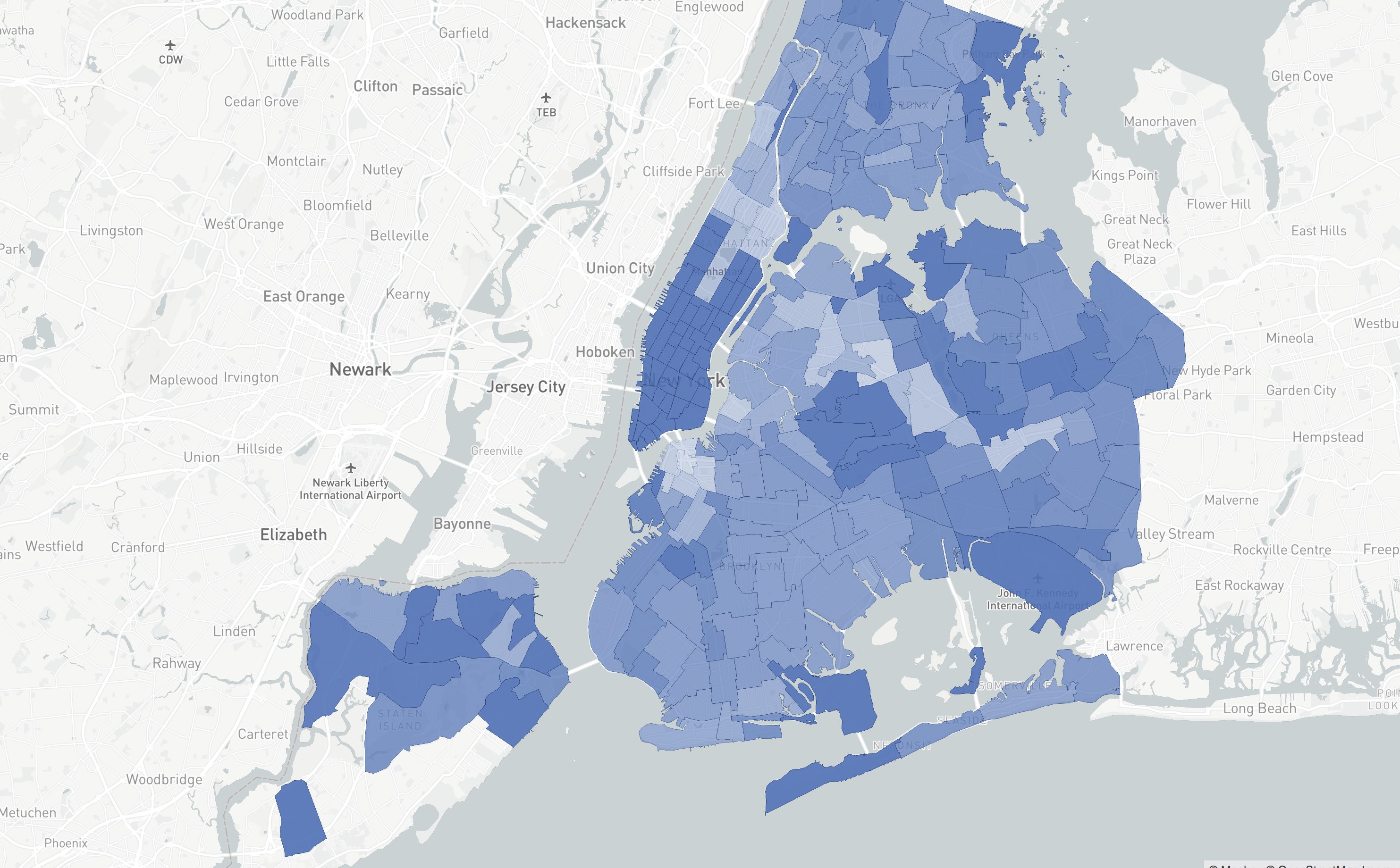
Here's a quick peek at the output of the model. The areas are shaded on a logarithmic scale according to their profitability. Hover over an area to see information about it.
Click here for a preview if the map doesn't load.
It's interesting to see what one would expect: Manhattan is profitable and so are the areas around airports: JFK (the large area in the bottom right hand corner) and LaGuardia. Note that the profitability does not really translate to a real dollar amount, it's more an arbitrary metric.
Background
A friend of mine recently brought to my attention the cool open data available from the NYC Taxi & Limousine Commission's site. There is some quite interesting data there, and I ended up thinking about good ways to model the profitability of certain areas in NYC, trying to figure out what kind of model would capture this well. This post is a quick overview of the model I came up with and how I went about solving it.
The data available on the TLC site consists of rows of data per-ride with fields including the dropoff and pickup date/location, the trip distance/duration/number of passengers, and the charge, fees, tip, etc. The dropoff and pickup locations are encoded as custom polygons that you can also download as a shapefile from their site.
A somewhat natural question to ask given this per-trip data, is: what's the profitability of some location?
There's quite a few ways of looking at this and trying to answer such an open ended question. For example, one may look at the time-series of how often a driver gets rides from different areas, and so on. However, the model I decided to go for was based rather on trying to understand how the destination area influenced the profitability of the current area. For example, suppose a taxi takes a passenger from Downtown Manhattan to somewhere in Brooklyn, but — for the sake of argument — riders in Downtown Manhattan tip a lot more than those in Brooklyn; then obviously this one-time trip may lead the driver to an area with low profitability. We want to capture this kind of dynamic and so chose a model where the profitability of a given area is influenced by the profitability of probable future locations.
To get some rough metric for profitability, we let the profitability of a ride be the total fare divided by the duration in minutes. I had to do some cleaning to get rid of data with very low durations (due to inaccuracy in timing).
Our model
Let \(\mathcal{S}\) be the set of (pickup/dropoff) areas, and let \(\mathcal{T}\) be the set of all trips. For \(i,j\in\mathcal{S}\), \(\mathcal{T}_{i,j}\) to be the set of trips from \(i\) to \(j\) and \(\mathcal{T}_i\) to be the set of trips originating from \(i\in\mathcal{S}\). For a trip \(e\in\mathcal{T}\), let \(p_e\) be its profitability.
We now define
\[ q_{i,j}=\frac{1}{|T_{i,j}|}\sum_{e\in\mathcal{T}_{i,j}}p_e, \]
the (empirical) expected profitability of a trip from \(i\) to \(j\). Similarly we define
\[ q_i=\frac{1}{|\mathcal{T}_i|}\sum_{e\in\mathcal{T}_i}p_e, \]
the expected profitability of a trip originating from \(i\).
Finally define
\[ w_{i,j}=\frac{|\mathcal{T}_{i,j}|}{|\mathcal{T}_i|}, \]
the expectation of the proportion of trips originating from \(i\) that go to \(j\).
Now let \(p_i\) for \(i\in\mathcal{S}\) be the (expected) profitability of an area. We wish for the vector of profitabilities to satisfy
\[ p_i=\sum_{j\in\mathcal{S}}w_{i,j}(q_{i,j}+\gamma p_j), \]
for some discounting factor \(\gamma\in(0,1)\). This says that the profitability of an area is the weighted average (by proportion of trips) profitability of destination areas plus some discounting factor times the profitability of that area. So if an area is average but often leads to a very profitable area, then the first area is also pretty good in the scheme of things.
Simplifying this, we can also write
\[ p_i=q_i+\gamma\sum_{j\in S}w_{i,j}p_j, \]
so the profitability of an area is the average profitability of outgoing trips plus the discounted weighted average profitability of destination areas.
Writing \(\mathbf{W}\) as the matrix of \(w_{i,j}\), and similarly \(\mathbf{p}\) and \(\mathbf{q}\) for the column vectors of \(p_i\) and \(q_i\), we get the matrix equation
\[ \mathbf{p}=\mathbf{q}+\gamma\mathbf{W}\mathbf{p}, \]
and rearranging, we have
\[ \mathbf{p}=(\mathbf{I}-\gamma\mathbf{W})^{-1}\mathbf{q}, \]
where \(\mathbf{I}\) is the identity matrix of appropriate size and the inverse is the matrix inverse.
Note that we need \(\gamma<1\) here (instead of having \(\gamma=1\)) because by construction, \(\mathbf{W}\) is a stochastic matrix, so \(\mathbf{I}-\mathbf{W}\) has vanishing row sums, so the rows are linearly dependent and \(\mathbf{I}-\mathbf{W}\) is singular. One can also see this intuitively from the model: in the presence of cycles — ways of starting from one area and then getting back there — the the weighted sum for \(p_i\) gives an infinite recursion, and one can see that having no discounting would be problematic.
This kind of model is called a Leontief Input-Output model.
The nitty gritty
I loaded the data into a Jupyter notebook and created a Pandas dataframe to hold the taxi data. After a few simple groupbys and aggs, I got the data I needed, put those in a Numpy matrix, and did a quick matrix inverse with numpy.linalg.inv to get the results.
import pandas as pd
import numpy as np

# import and cleaning
df_raw = pd.read_csv("green_tripdata_2020-01.csv")
df_raw["p"] = df_raw.total_amount / ((pd.to_datetime(df_raw.lpep_dropoff_datetime) - pd.to_datetime(df_raw.lpep_pickup_datetime)) / np.timedelta64(60, "s"))
df = df_raw[["PULocationID", "DOLocationID", "p"]].rename(columns={"PULocationID": "pickup", "p": "p_e", "DOLocationID": "dropoff"})
df = df[(df.p_e > 0) & ~df.p_e.isna() & (df.p_e < 10)]

# list of all locations/areas, having dropoff areas with no pickups causes issues with the weight matrix
areas = df.pickup.unique()
df = df[df.pickup.isin(areas) & df.dropoff.isin(areas)]
ix_lookup = {val: ix for ix, val in enumerate(areas)}
n = len(areas)

# creating the T_{i,j} matrix
Tij = np.zeros([n, n])
for (i, j), val in df.groupby(["pickup", "dropoff"]).agg("count").p_e.items():
    Tij[ix_lookup[i], ix_lookup[j]] = val

# computing the W matrix...
W = (Tij / Tij.sum(axis=1)).T

# ...and q vector
q = np.zeros([n])
for i, val in df[["pickup", "p_e"]].groupby("pickup").agg("mean").p_e.items():
    q[ix_lookup[i]] = val

# set it pretty high
gamma = 0.6

# compute p
p = np.linalg.inv(np.eye(n) - gamma * W) @ q

# save to csv
with open("p.csv", "w") as f:
    f.writelines(f"{areas[i]},{val}\n" for i, val in enumerate(p))
I then imported the shapefile taxi zone areas into PostGIS with ogr2ogr:
ogr2ogr -overwrite \
  -nln areas \
  -nlt PROMOTE_TO_MULTI \
  -nlt MULTIPOLYGON \
  -lco CREATE_TABLE=YES \
  -lco GEOMETRY_NAME=geom \
  out.sql \
  taxi_zones.shp
cat out.sql | psql
Finally I exported the \(\textbf{p}\) vector into PostGIS and did a spatial join against the shapefiles from T&LC's site to get the following dataset.
create table values(
  locationId int not null,
  p real not null
);
-- \copy is a psql built in command that allows access to the local fs
\copy values(locationId, p) from 'p.csv' with csv;
select * into taxi_profitability from (
  select geom, shape_area, zone, values.locationid, borough, p
  from areas
  inner join values
  on values.locationId = areas.locationid
) t;
Then export it into GeoJSON (we need to reproject to EPSG4326, I'm not sure what the original SRS is, something NYC specific, it seems)
ogr2ogr -t_srs "EPSG:4326" taxi_profitability.geojson PG:"tables=taxi_profitability"And that's it, now just load it into a map or into QGIS and you can look at the pretty colors!